Aerodynamic performance of spherical tires vs conventional tires

In the future Goodyear estimates to replace it's conventional cylindrical tires with Eagle 360 concept spherical tires for driver less vehicles. By the use of magnetic levitation, the spherical tires are expected to be connected to their vehicles. With this tire design, drivers can ignore pot holes, since, the vehicles are expected to stay afloat. If necessary, each spherical tire is also capable of rotating independently and providing the vehicle to travel laterally.

Sensors are embedded into these spherical tires to automatically collect data regarding road conditions, tire wear, weather conditions, traffic data, tire pressure level etc. Gathered data by this sensor is then transferred to the AI of the spherical tire and it is then supposed to analyze and translate this data to the betterment of the tire and automobile. For instance, the tire transforms itself into a smooth surface if it's sensors determine a dry pavement road. While driving wet roads, the tires deploy grooves that acts as sponge to reduce the chances of hydroplaning.

The spherical tires rotate smartly to increase its overall lifespan. Magnets are installed around the spherical tire to control its braking, acceleration and rotation. Based on

above mentioned features, the Eagle 360 spherical tire promises to be convenient and

flexible for the passenger. Goodyear believes that this design will be the future of the

automobile tires. However, aerodynamics of these tires are not yet evaluated. Thus, the present research explores the aerodynamic characteristics of the spherical tires and compares its performance to today's conventional tires.

Aerodynamic performance of the spherical tires are numerically approximated at Re=5.3x10^5, based on the diameter of the tire. Utilizing ANSYS Fluent, various simulations are performed and aerodynamics of the spherical tires are estimated using k-transition turbulence model. SIMPLEC algorithm and second order upwind scheme are used to solve and discritize the turbulent and momentum equations. Below mentioned steps are followed in sequence to construct a 3-D computational domain and to perform the numerical simulations.

1) Geometry and enclosure

The 3-D spherical tire is designed using Solid Works. To reduce finite volume mesh complexity, the spherical grooves of the spherical tire are replaced with cylindrical grooves (see Fig. 1.1-1.2). Furthermore, the hexagonal faces are removed to obtain a simplistic geometry.

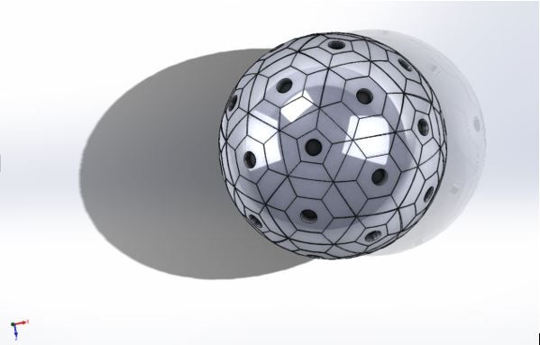
Figure 1.1: Spherical tire with hexagonal faces and spherical grooves

Figure 1.2: Spherical tire with cylindrical grooves

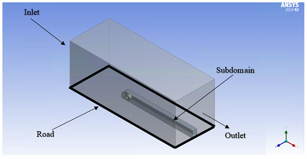
A 3-D enclosure with subdomains are built around the spherical tire using Ansys design modeler.

For the present study, two spherical tires, grooved and smooth spherical tires, are chosen. The drag coefficient for the two spherical tires is evaluated to analyze the in Cd due to the grooves of the tire. Drag exerted on the these spherical tires is evaluated for numerous cases for instance, case 1A (isolated stationary spherical tire), case 1B (isolated rotating spherical tire) and case 2 (rotating spherical tire in the presence of rigid ground). Cd of the smooth and grooved spherical tire are also compared to the Cd of conventional tires.

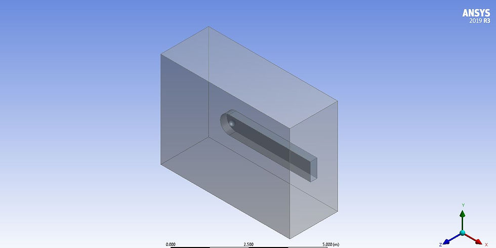
Figure 1.3: Enclosure for cases 1 and 2

Figure 1.4: 3-D enclosure with subdomain for case 2

2) Mesh

A 3-D structured mesh is generated using ANSYS Mesh software (an ANSYS Workbench tool). A cut cell approach is used to generate this mesh (see Fig. 2.1-2.2).

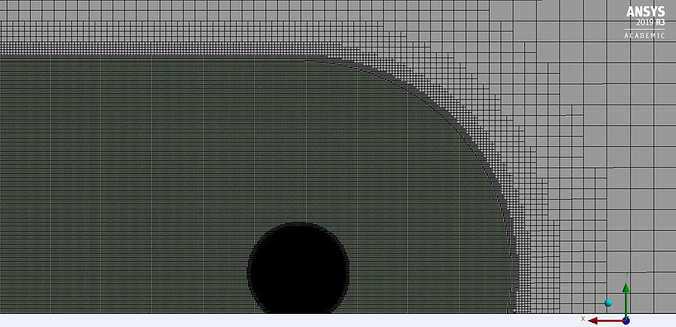
Figure 2.1: Structured 3-D cut cell viewed in plane parallel to the airflow

Inflation layers are generated around the spherical tire to capture the turbulent wall bounded effects.

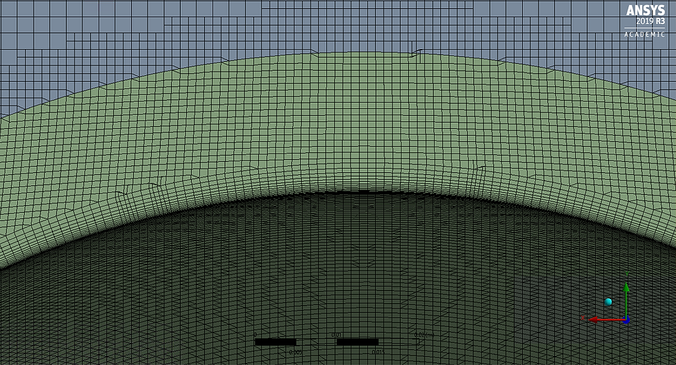
Figure 2.2: Inflation layer mesh around the spherical tire aligned with the outer structured grid

By calculating the Y+ and delta y, the inflation layer mesh around the spherical tire is generated

Re_L= ρUL/μ

U_τ=√(τ_ω/ρ)

τ_ω=1/2 ρU^2 * CF

CF =0.058Re^(-0.2)

y+ = (ρU_τ△y_1)/μ

Where L is the characteristic length, CF is the coefficient of friction, U_τ is the frictional velocity, △y is the first layer height and y+ is the non dimensional wall distance.

Required no of inflation layers is calculated to achieve a smooth transition of mesh between the inflation layer and the outer structured grid.

Vertical surfaces are generated in between the spherical tire and road (see Fig. 2.3), for case 2, to eliminate the non-orthogonal mesh elements (dirty geometry).

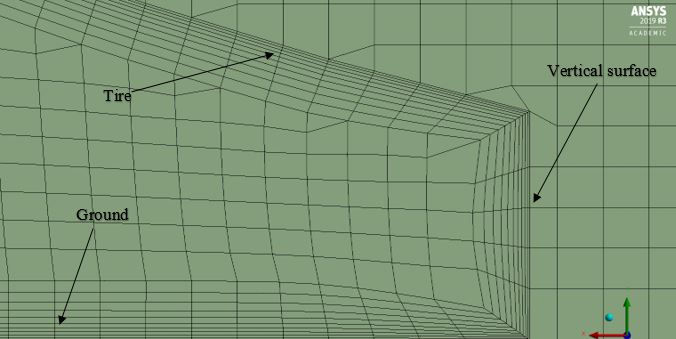
Figure 2.3: Inflation layers mesh alignment near the contact patch

Inflation layers are also generated inside the grooves (see Fig. 2.4) of the spherical tire to capture the airflow inside the grooves.

Figure 2.4: Inflation layer mesh inside the grooves of the spherical tire

3) Boundary conditions

Inlet boundary condition for the inlet face for all cases

pressure outlet boundary condition for the outlet face for all cases

Slip wall boundary condition to the top and side walls of the enclosure for case 2

All walls except for the inlet and outlet are assigned with slip boundary conditions for cases 1A and 1B

Moving wall boundary condition to the road for case 2

Rotating boundary condition to the spherical tire for case 2 and case 1B

No slip boundary condition is assigned to the spherical tire for case 1

4) Results

Due to grooves of the spherical tire, the drag coefficient increased by 107.9% for isolated stationary spherical tire. However, due to the grooves of the spherical tire, the drag coefficient increased by only a 22% and a 36% for isolated rotating spherical tire and rotating spherical tire in the presence of moving ground (see Table 4.1).

The drag coefficient acting on the spherical tire is further analyzed by evaluating the increase in the skin friction and pressure coefficient values due to the grooves for all cases

Table 4.1: Increase in pressure and skin friction coefficient for all cases at Re=5.3x10^5

% increase in pressure coefficient % increase in skin friction coefficient

Case 1A 112.8% 5.2%

Case 1B 12% 18.6%

Case 2 0.7% 96%

The increase in pressure coefficient for cases 1A and 1B are analyzed by plotting and comparing the static pressure contours at the mid cross section. The skin friction coefficient is further dissected by analyzing and comparing the wall shear contours on the surface of the grooved and smooth spherical tires.

For isolated stationary spherical tire, a low pressure region on the downstream side and a high pressure region on the upstream side of the spherical tire is occurred (see Fig. 4.2). Furthermore, we also observe an additional pressure force due to the grooves of the spherical tire (see Fig. 4.2). This will further increase the pressure drag of the isolated stationary grooved spherical tire.

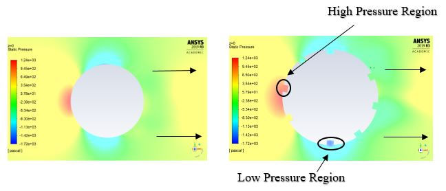
Figure 4.2: static pressure contour at Re=5.3x10^5 for case 1A

For case 1B (rotating isolated spherical tire), a lower magnitude of low pressure region is observed for grooved spherical tire compared to smooth on the downstream side (see Fig. 4.3). Furthermore, the grooves of the spherical tire also contributes to additional pressure drag compared to the smooth spherical tire, for case 1B (see Fig. 4.3).

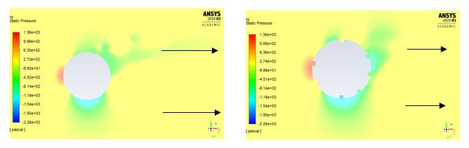
Figure 4.3: Static pressure contours at Re=5.3x10^5 for case 1B

Wall shear contours, when plotted on the surface of the spherical tires, indicate formation of additional wall shear force behind the grooves of the spherical tire, for case 1A (see Fig. 4.3-4.4).

Figure 4.3: upstream side wall shear contours at Re=5.3x10^5 for case 1A

Figure 4.4: Side view of the wall shear contours at Re=5.3x10^5 for case 1A

A higher wall shear region is witnessed on the upstream side of the grooved spherical, compared to the smooth for rotating isolated spherical tire (see Fig. 4.5).

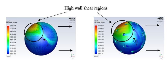
Figure 4.5: Side view of the wall shear contours at Re=5.3x10^5 for case 1B

Figure 4.6: Upstream side wall shear contours at Re=5.3x10^5 for case 1B

The wall shear contours also indicate a high wall shear region on the top and lower wall shear region on the bottom of the rotating grooved spherical tire in the presence of the road, compared to smooth (see Fig. 4.7-4.8).

Figure 4.7: Top view of the wall shear contours at Re=5.3x10^5 for case 2

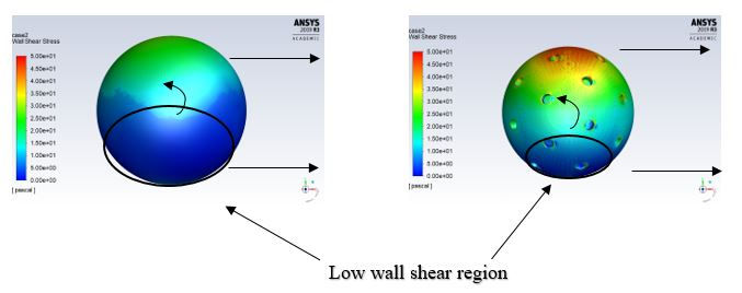
Figure 4.8: Side view of the wall shear contours at Re=5.3x10^5 for case 2

Drag coefficient of the spherical tires vs conventional tire

Numerous simulations with k-transition turbulence model, SIMPLEC algorithm and second order upwind scheme are used to study the drag exerted on the rotating conventional tires in the presence of road. Results from these simulations indicated that the drag coefficient of the spherical tire, regardless of the grooves, decreased by 107.9%, compared to the conventional tires. But this does not mean that the spherical tires are aerodynamically superior to the conventional tires, since drag force is used to judge the aerodynamic efficiency of the tire rather than drag coefficient. Furthermore, drag force is related to the reference area of the geometry (tires). The reference area of the spherical tires is pi*r^2 but for conventional tires it is length times the diameter. This indicates that the reference area for the spherical tire is less than half of that of the conventional tire. This leads to a drag coefficient less than half for the spherical tires compared to the conventional tires. In conclusion, one can state that the aerodynamic efficiency of the spherical tires are comparable to the conventional tires.

References

[1] Pakala, A. K., 2020, "Aerodynamic Analysis of Conventional and Spherical Tires," MS. c thesis, University of Akron.

Important note: Information, pictures, graphs, tables and data presented in this blog is borrowed from Akshay Kumar Pakala's Master's thesis document.